
A Bayesian Approach to Filtering Junk E-Mail - Part 1


Bayesian spam filters are generally known at a popular level in knowledgeable tech circles. I believe Paul Graham made it better known in these groups long back. I have vague recollections on the topic from a decade or so ago. The paper in question “A Bayesian Approach to Filtering Junk E-mail” was done in 1998 by a collaboration between researchers in Stanford and Microsoft Research.
You can see elaborate descriptions of what spam email is, where it originates from and so on - highlighting the level of familiarity with the “spam phenomenon” back in the day. People started building up rules to block spam. They said - if it comes from email X - block it or delete it and so on. Or they said if it contains Y and Z keywords - delete it. But the researchers noticed that this is too rigid a model - because rulesets are binary or black and white. The authors wanted a probability number providing a degree of confidence factor for classification - rather than a binary result.
An important point the authors held to was a clear understanding of the trade-offs involved. They say - it’s alright if we get an occasional spam in the inbox - as long as we don’t miss any genuine email. That is, the cost of misclassifying genuine email is more than the cost of misclassifying spam.
Anyway - my purpose here is a bit more remote. I want to learn the underlying thinking and framework - quite a bit of it of a mathematical nature. So I will be trying to grasp at these concepts through a series of posts. Hopefully it turns out to be both interesting and fruitful.
Bayesian Networks
The underlying mathematical structure from which Bayesian Spam Filters were invented is called Bayesian Networks. It was Judea Pearl - who was a major figure in pushing the idea of Bayesian Networks forward. Something like:
A -> B
A is a random variable. B is a random variable. A (parent) influences B (child).
What is the point of Bayesian Networks? It helps us represent “join probabilities” in an easy-to-understand way. Joint probability means - there are multiple connected events that need to be represented, and we are interested in the probability of each happening, based on the probabilities of the other related events. Bayesian Networks make it possible for us to put these events and probabilities into a graph (a Directed Acyclic Graph) and a table of probabilities.
In the real world - where many events happen, with all sorts of sequences - we end up with complex graph representations. How does Bayesian Network (BN) ideas help us cope?
The core idea in BN is that not every variable or node depends on every other variable. Most relationships in the real world are local. One node influence only the nearby nodes, and those nodes in turn affect further neighboring nodes - like ripples pushing through water.
Nodes, Parents, Arrows
BN is a Directed Acyclic Graph (DAG, as is commonly known in CS)
Each node is a random variable.
Each arrow is an influence - that is parent helps “determine” the child.
Example:
Rain → WetGrass → Slip
This says: Rain affects whether the grass is wet, and wet grass affects whether someone slips.
Parents Explain the Node (if They’re Known)
BN is governed by the “local Markov Property” which says something like:
Once you know a node’s parents, nothing else in the network can help you predict that node any better.
This is the heart of the entire theory.
It tells us that all the information needed to determine a variable is already captured in its parents. Once the parents become known, there is no better way to determine the node than via the parents.
For example, if you know whether it rained and whether the sprinkler was on, then:
the stock market,
the temperature,
or whether someone slipped
add no new information for predicting whether the grass is wet.
The direct causes are enough.
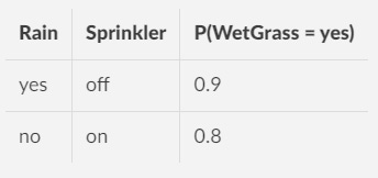
Conditional Probability Tables (CPT)
Another technical component of BN is the Conditional Probability Table (CPT).
It defines the parents of a node, and the node itself. It mentions the state of the parents, and then gives a probability for the present node.
BN is concise - because each n ode has its own table - there is no need to look at all the other nodes and their concerns. CPT is a focused and simple device at the nodal level.
How BN simplifies Joint Probability Calculation
By sticking to “parents explain the node”, BN simplify the calculation for joint probability significantly:
This factorization:
makes learning easier,
makes inference faster,
and lets us model complex systems with far fewer parameters.
In Conclusion…
A BN is a directed graph where arrows represent influence.
Each node depends only on its parents.
Once parents are known, the node is mathematically “sealed off” from the rest of the network.
This lets us represent huge probability distributions using small local tables.
Thus, a DAG becomes a compact and powerful probabilistic model useful in many domains of interest to humanity.