A Neural Image Caption Generator - Part 4

Quick Recap

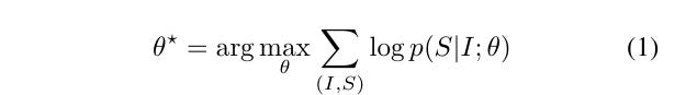
Yesterday we saw equation (1) in detail - where we try to pick the best θ

Decompressing Eq (1)

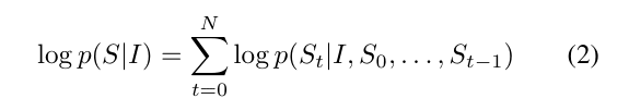
While that is the conceptual representation - in practice - we use equation (2)

Here S is:

\(S \;\;=\;\; (S_0, S_1, \dots, S_N)\)

S the sentence as a whole. It is a single random variable which represents “all finite-length sentences”

\(S_t \;\;=\;\; \text{the } t\text{-th coordinate of } S\)

Concretely:

• S_t​ is one symbol in the sequence

• Typically: a word, subword, or token

So:

\(p(S \mid I) = p(S_0, S_1, \dots, S_N \mid I)\)

This is a joint probability over a variable-length object.

As written, it is:

• mathematically valid

• computationally useless

Equation (2) exists to make this representable.

We apply the chain rule to get:

\(p(S_0, \dots, S_N \mid I) = \prod_{t=0}^N p(S_t \mid I, S_0, \dots, S_{t-1})\)

Taking logs, we get:

\(\log p(S \mid I) = \sum_{t=0}^N \log p(S_t \mid I, S_0, \dots, S_{t-1})\)

How Eq. (1) → Eq. (2) should be read together

• Eq. (1):
  “Maximize the probability of correct sentences given images.”

• Eq. (2):
  “Here is how that sentence probability decomposes internally, without approximation.”

Once the mathematical representation is done, we move to the first place where a real modeling approximation enters.

Up to Eq. (2) everything was exact. Eq. (3) is where the engineering starts.

From Eq. (2) we need to model:

\(p(S_t \mid I, S_0, \ldots, S_{t-1})\)

This conditional depends on:

• the image I

• an unbounded, growing history of tokens

This is not directly representable.

So the question becomes:

How do we compress (I,S₀,…,S_t−1)(I, S₀, …, S_t-1) into something finite and computable?

Making Eq (2) Computable (approximately)

The paper assumes:

All relevant information from the past can be summarized in a fixed-length state h_t

Formally:

\((I, S_0, \ldots, S_{t-1}) \;\longrightarrow\; h_t\)

This is not exact.
This is the approximation.

What Eq. (3) states

\(h_{t+1} = f(h_t, x_t)\)

Meaning:

• h_t: current memory (summary of everything seen so far)

• x_t​: the new input at time ttt

• f: a learned nonlinear update rule

This defines a recursive state update.

Nothing probabilistic yet — this is a state machine.

What is x_t?

This is deliberately abstract here.

Later they specify:

• at t=0: x₀ includes image features (from a CNN)

• for t>0: x_t is an embedding of S_t−1

So:

• the image is injected once (or early)

• words are fed in sequentially

Once you have h_t, the model defines:

\(p(S_t \mid I, S_0, \ldots, S_{t-1}) \;\approx\; p(S_t \mid h_t)\)

Typically, via:

\(p(S_t \mid h_t) = \text{softmax}(W h_t)\)

This approximation is the heart of the RNN approach.

Why an RNN / LSTM specifically

• RNN: implements the recurrence in Eq. (3)

• LSTM: a particular choice of f that resists information loss over long sequences

How Eq. (3) fits in the narrative:

• Eq. (1): what to optimize

• Eq. (2): how sentence probability decomposes

• Eq. (3): how we approximate the required conditionals

Eq. (3) is the bridge from probability to neural networks. Equation (3) says: “Replace an ever-growing history with a single evolving memory vector.”

This is where mathematical expressiveness is traded for computational tractability - -deliberately and explicitly.