
Building the Unix Spelling Corrector from Scratch - Part 2


Candidate corrections obtained via edits. An edit can be:
Insert
Delete
Substitution
Reversal
The authors got their “edits dataset” from news orgs - where news has to be shipped under tight deadlines.
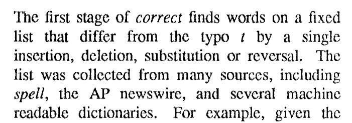
Now we look at an example. Consider a mistyped word, acress. We try to figure out some potential correction candidates, which with a few transformations lead to the mistyped word.
Say we start with the correction candidate actress. We have at index 0, the character a. Index 1, character c. And Index 2, the character t. What is required is - we should delete this character t at index 2. If we do that, we get the mistyped word acress. We can put that transformation more formally as: “@ t 2 deletion”. @ means a null in the typo. Something is missing there. And with deletion to the correction we are fixing.
Let’s take one more example. Consider the candidate cress. Here, at index 0 , we have the character c. In the mistyped word, we start with a. So the solution is we must insert a at index 0. This can be represented as “a # 0 insertion”. Here, “#” means - null in the correction side.
In this way - we can come up with many types of “correction candidates” based on the typo:

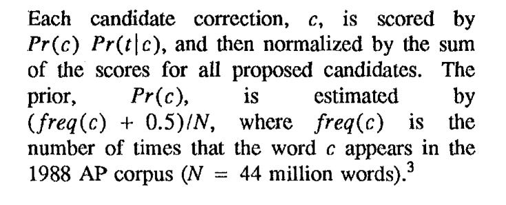
For each candidate correction - we calculate P( c) P(t|c).
P( c) is mainly about the “frequency” of the given correction in the corpus. But we use Jeffrey’s Prior or add 0.5-smoothing used in Bayesian estimation for multinomial (or binomial) proportions.
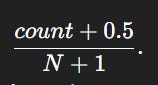
The intuition for Jeffrey’s Prior is this:
Before seeing any data, I want a prior that doesn’t bias the probability toward any particular word, but still prevents zero probabilities.
It adds a small amount—less than Laplace’s +1—so rare words aren’t inflated too much.
The formula for Jeffrey’s prior is like this:
But for the spell correction model we use:
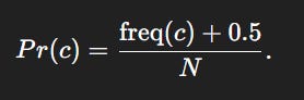
We ignore the +1 in the denominator since N = 44 M, so the +1 is negligible.
The formula effectively:
avoids zero probabilities for unseen words,
doesn’t distort the distribution as much as Laplace smoothing,
is mathematically grounded.
The next section requires knowing what “bigram” means. It’s simply “two characters that appear next to each other in text”.
Consider the word “cat”. The bigrams are “c a” and “a t”.
We need to define the four cases discussed above with a bit more detail:
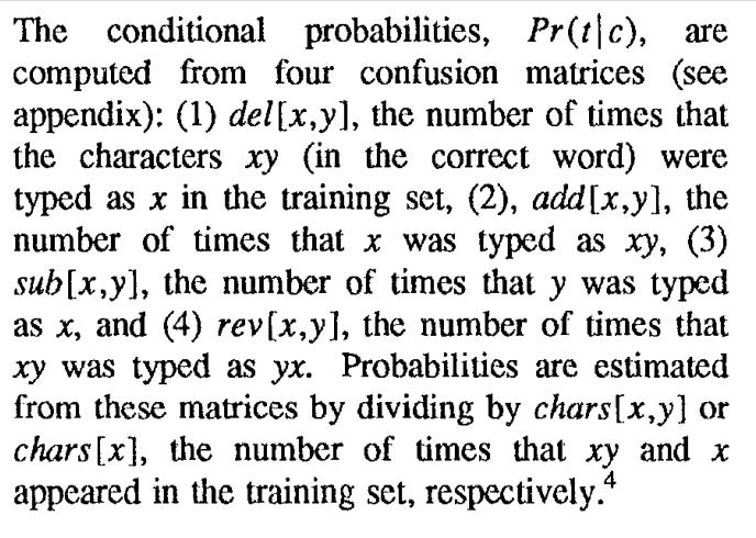
Deletion: del[x,y] means - number of cases where “xy” was intended, but actually only “x” was typed in the training set
Addition: add[x,y] means - number of cases where “x” was intended, but actually “xy” was typed in the training set
Substitution: sub[x,y] means - number of cases where “y” was intended, but “x” was typed
Reverse: rev[x,y] means - number of times that xy was typed as yx.
The above gives various “frequencies”. To get probabilities we divide by the number of times xy or x appeared in the training set - as chars[x,y] or chars[x]
The cases can be put like this in mathematical form:
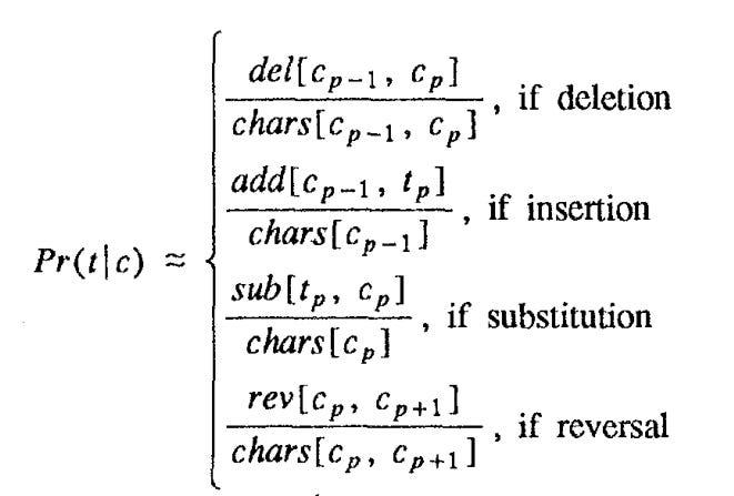
The denominators basically represent “correct typing'“, and the numerator “mistaken typing”. Case 1 - deletes the second letter/parameter. Case 2 - a false letter is added at the end. Case 3 - a false letter is typed instead of the expected one. In reversal, Case 4 - the order is messed up.
Based on the above formula - we have to calculate the 5 matrices (4 from above cases, and one from the general case). We start with uniform distribution over confusion, run each word through spell, create correction candidates, and iteratively update the confusion matrix. Then smooth the matrices using Good-Turing method