
Reimplementing Unix correct: The Lost Bayesian Spelling Corrector

The Problem
Last week, I worked through a classic paper in the Applied Bayesian tradition: The Unix Correct Program paper, built on noisy channel Bayesian foundations.
My goal was to work through the paper and reconstruct a spelling corrector similar to correct.

Along the way, I had to contact the original author, Prof. Kenneth, to find some data and code - turns out the full implementation of the correct program has been lost in the tides of time.
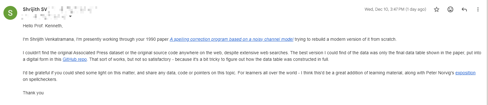
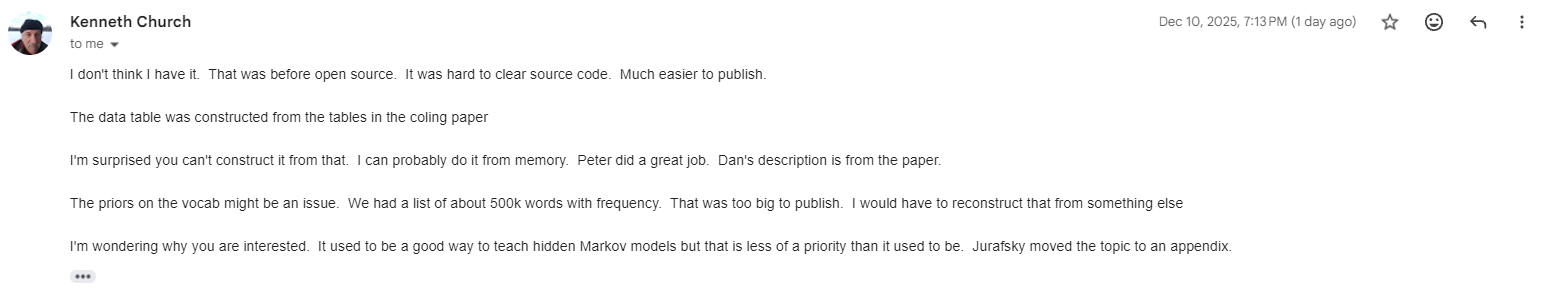
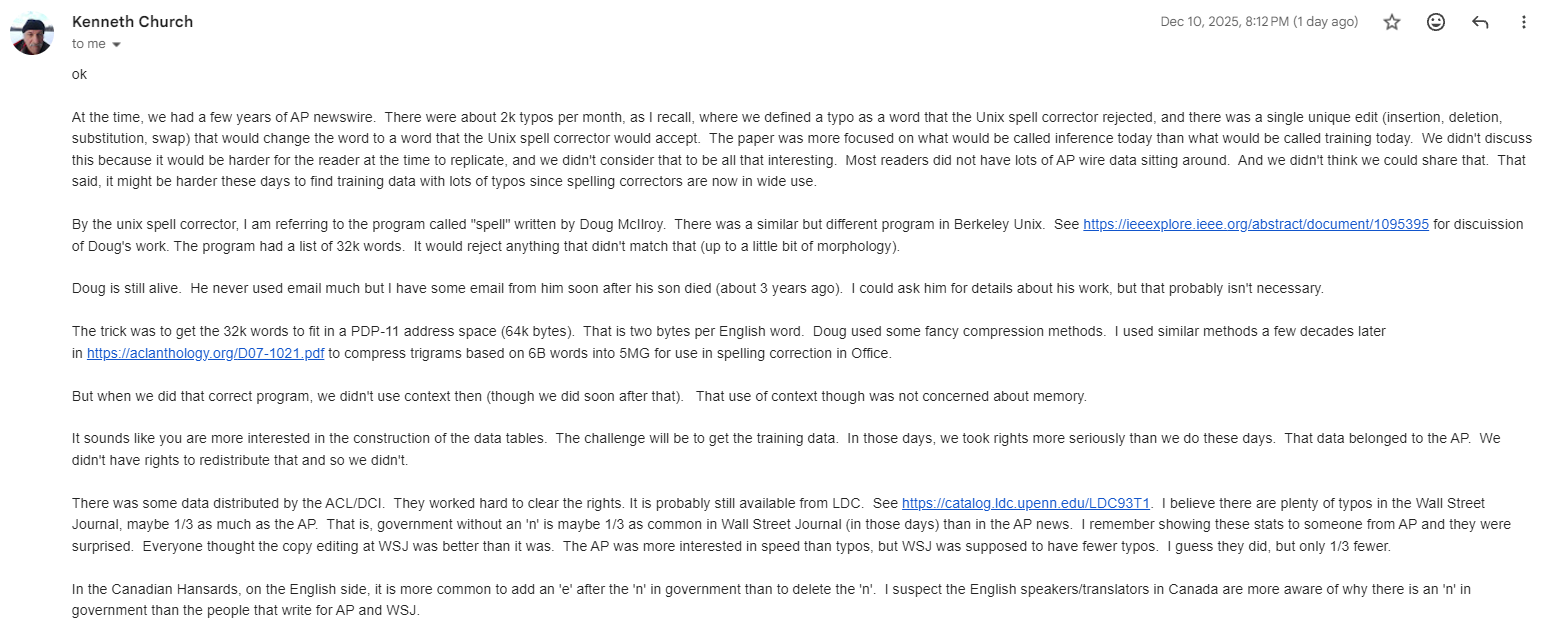
So, it fell upon my shoulders to imagine how it might have worked, and try to reconstruct something that functions similarly in principle.
Thankfully, I had some recovery work already done by Jaideep Bhoosreddy, in his GitHub repository aptly named spellcorrect.
The bulk of my implementation, the data, and so on is - thanks to Jaideep.
My contribution here is to use easier to understand functional constructs, to refine the presentation a bit more to help with understanding.
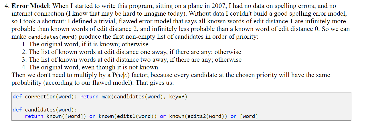
At the end of this - you can compare the implementation to Norvig’s implementation (which I also take a look at, as part of the series). You will find that the present implementation includes a nice, usable error model as part of the assessments. Norvig himself mentions that his implementation ignores the error model (instead - he relies on a simple edit distance mechanism):
The Full Solution
You can find the full re-implementation of the Unix spelling corrector in this Jupyter Notebook. I’ll walk you through some of the more important parts of it in the following section to give you a sense of how it works.
Concepts
We will use the following ideas or concepts along the way - and each of these will be explained from scratch with simple Python implementation:
N-gram language modeling
Noisy Channel Modeling and Bayesian Application
Error Confusion Matrices
Damerau-Levenshtein Edit Distance
1. Dependencies
Our implementation will be pure Python - with minimal dependencies. We use the “ast” module for loading the confusion matrix dataset from Jaideep (basically the dataset is available as raw python dicts). The Counter class is used for managing word counts/frequencies:
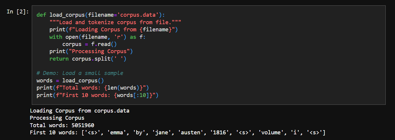
2. The Corpus
The original raw corpus can be found here - WARNING - it’s a big file!
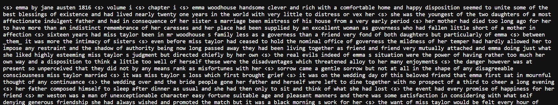
It looks something like the following - probably some cleaned up version of Emma by Jane Austen. We see everything in small case, no punctuation, etc - so there’s been some preprocessing.
We just load it and get an array of words:
3. Creating N-grams
An N-gram is a technical way of saying “phrases with N words”. Essentially - we pick up N sequential words from our corpus, try to find out how many times they appear in it.
unigram = 1-gram = single word
bigram = 2-gram = two sequential words from corpus
trigram = 3-gram = three sequential words from corpus
and so on.
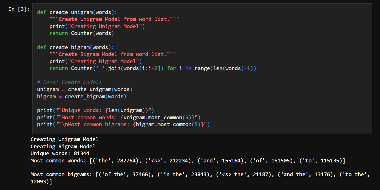
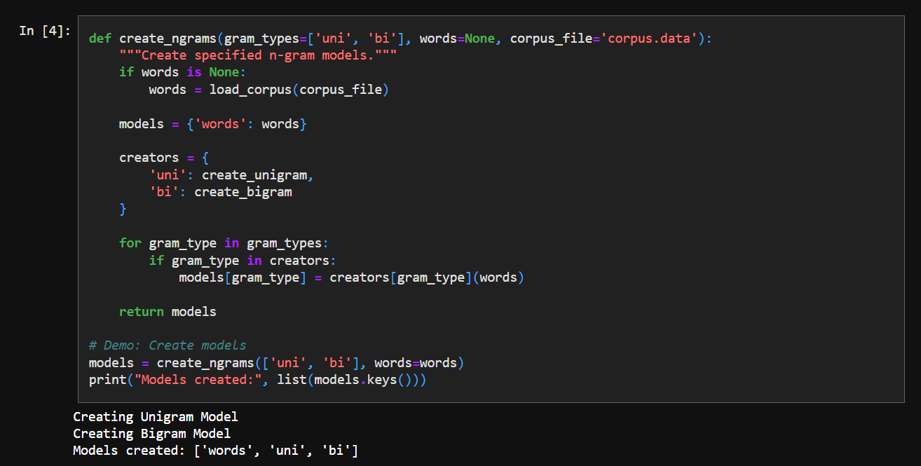
We organize the n-grams into a nice dict structure:
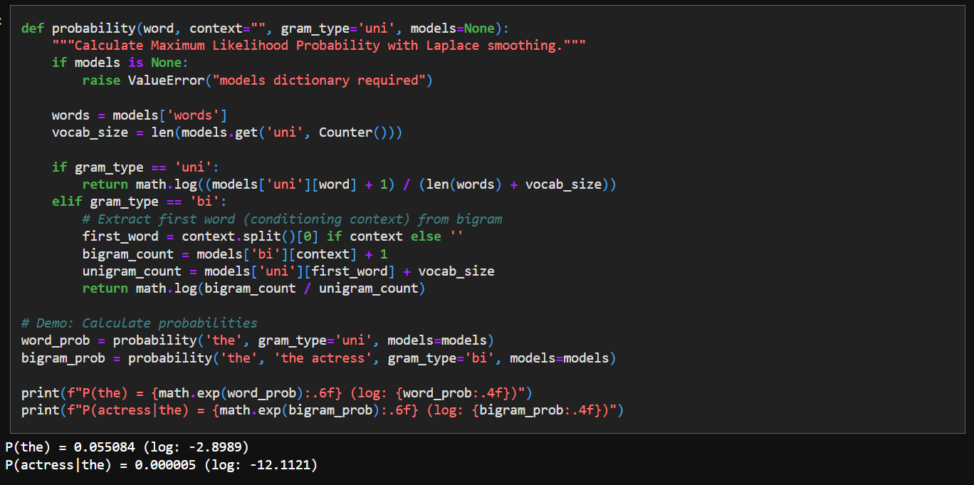
4. Calculating Probability
This function essentially turns raw word counts into usable probabilities.
It relies on two ideas:
the likelihood of a word can be estimated from how often it appeared in the corpus
the likelihood of a word given a previous word can be estimated from how often that pair appeared.
Our text source is just Emma by Jane Austen, some valid words or word pairs may never appear - so it’s just a rough approximation.
Laplace smoothing fixes these missing cases by assigning every possible word a small non-zero probability. This way, the model is able to handle phrases or sentences not seen before in the corpus.
We use log calculation to avoid numerical underflow in Python.
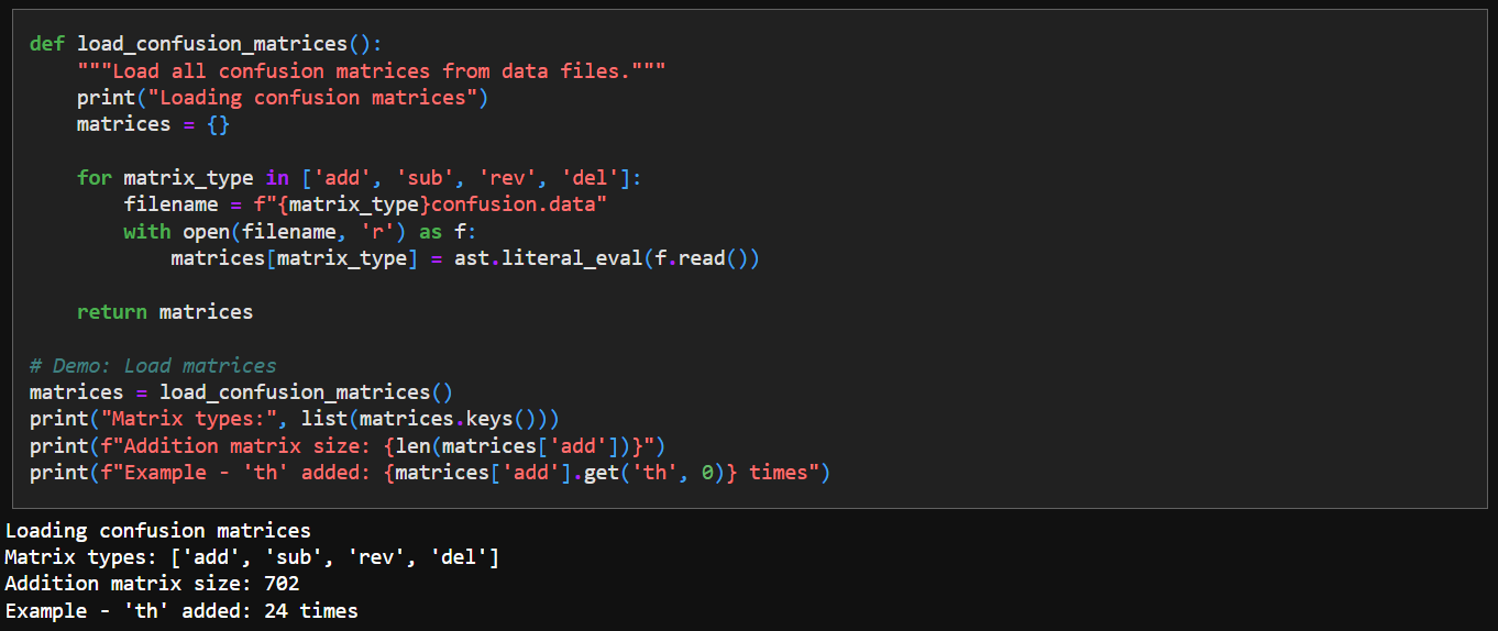
5. Load Confusion Matrices
The original paper published 4 confusion matrices for deletion, addition, subtraction, reverse for a pair of characters. Jaideep has converted them to a dict we can use:
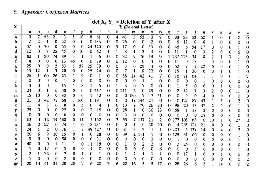
We come up with some simple loader code to import these tables:
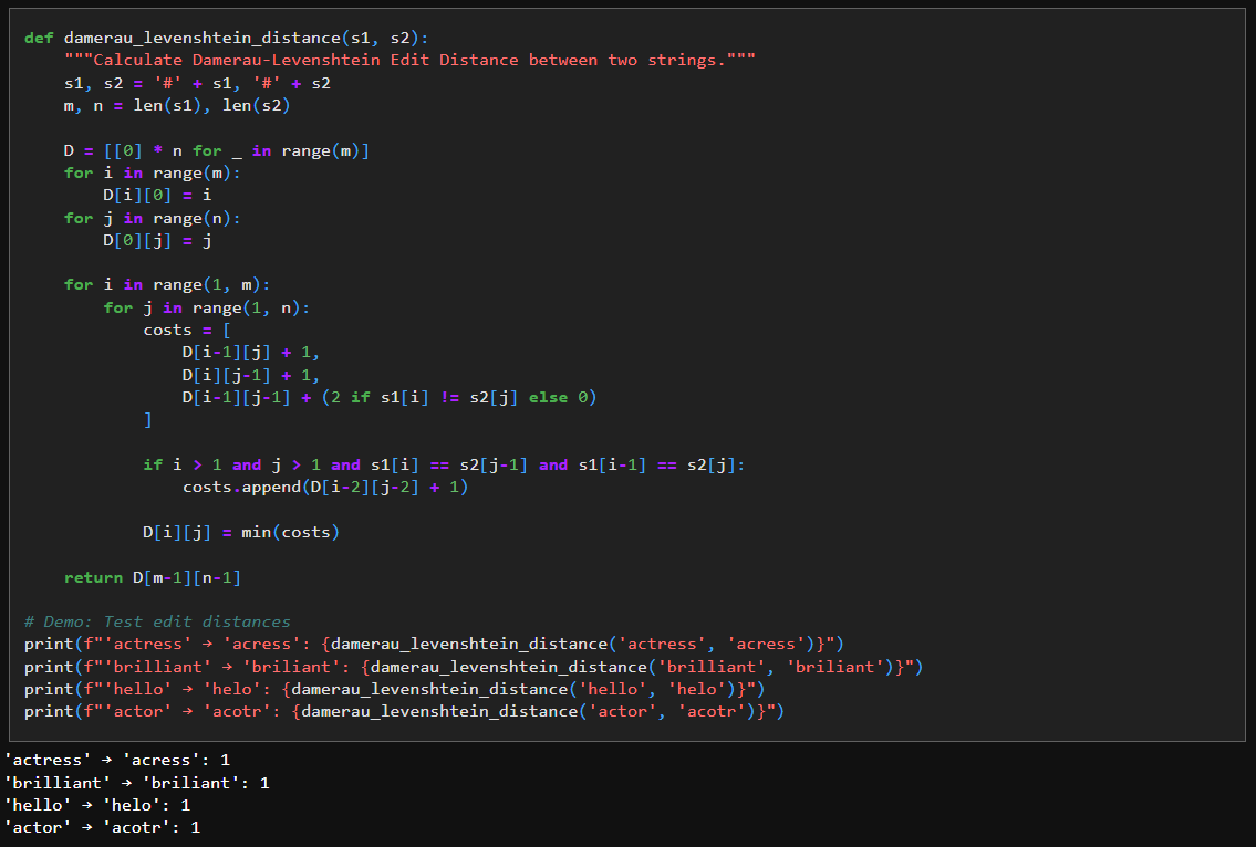
6. Edit Distance Function
We use Damerau-Levenshtein Edit Distance to find who similar/different two strings are.
The function works by comparing the two strings one character at a time and keeping track of the cheapest way to turn one into the other as it goes.
It first adds a dummy character (#) to the front of both strings so that index 0 naturally represents “no characters yet”, which simplifies the boundary logic.
The 2-D list D is then created to store costs: D[i][j] means the minimum number of edits needed to turn the first i characters of s1 into the first j characters of s2.
The first row and column are filled with increasing numbers because converting a word into an empty string (or vice versa) can only be done by deleting or inserting characters one by one.
For every remaining position, the code tries three concrete actions: delete a character, insert a character, or replace a character, and computes the cost of each using already-computed entries in the table.
If the current characters match, replacement costs nothing; if they differ, it costs more, which is why the code adds 2.
The extra check that looks two positions back handles a common typing mistake where two neighboring letters are swapped; when this pattern is detected, the code allows a cheaper transformation using a single operation.
By repeating this process systematically and always choosing the smallest cost, the final value returned represents the fewest edits consistent with the rules encoded in the code.
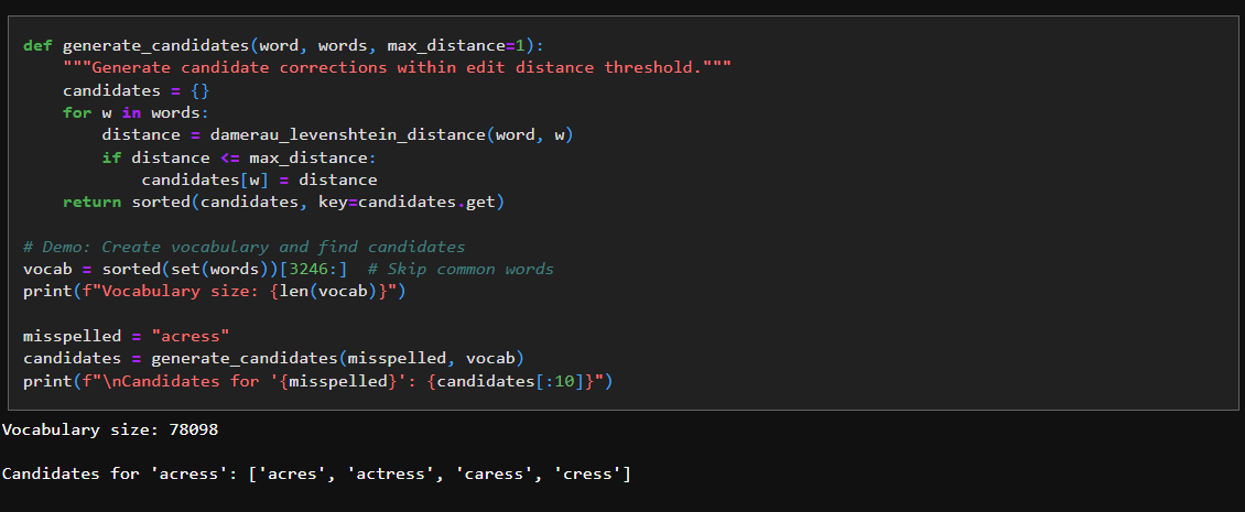
7. Generate Candidate Corrections
We use the edit distance logic above to generate candidate word options - given a word that needs fixing:
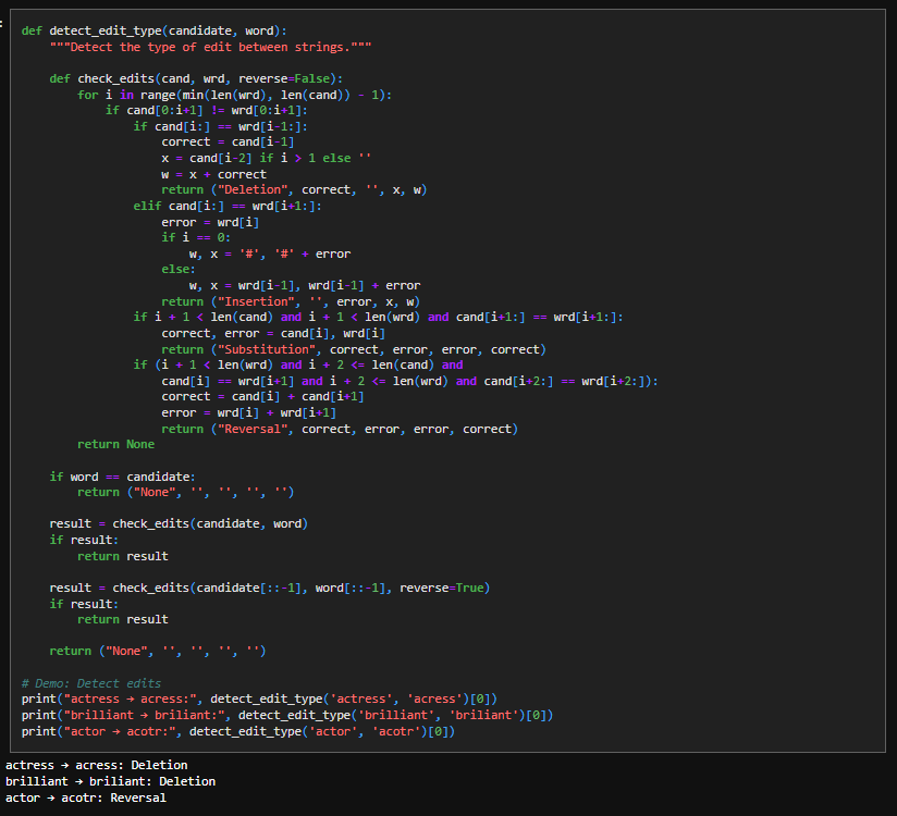
8. Detect Edit Types
This function tries to explain how one word could have turned into another by scanning from left to right until it finds the first position where the two strings disagree. At that point, it tests a small, fixed set of hypotheses that correspond to common typing errors: if skipping one character in the candidate makes the rest line up, it labels the change as a deletion; if skipping one character in the target word makes them line up, it is an insertion; if both strings realign after one character, it is a substitution; and if two adjacent characters appear swapped, it is marked as a reversal. Each test is implemented directly as a string slice comparison, which is why the code checks equality of the remaining suffixes rather than using distances. If no explanation is found when scanning forward, the function repeats the same logic on the reversed strings to catch errors that occur near the end of the word. The result is not a numeric distance, but a concrete edit explanation that identifies the error type and the characters involved.
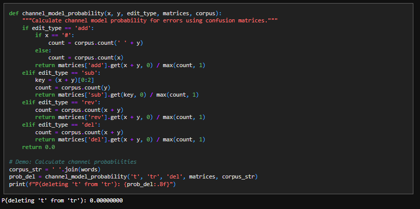
9. Channel Model Probability
This is essentially a lookup function for our confusion matrices:
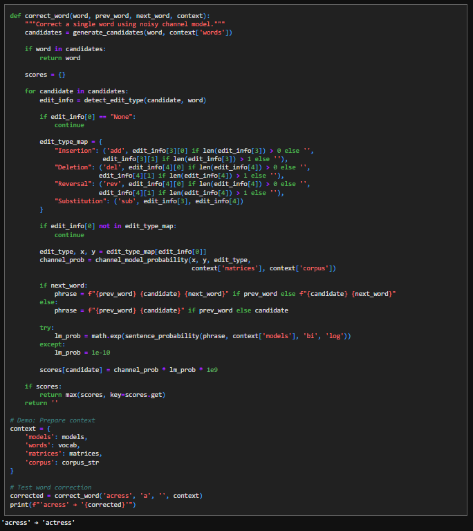
10. Word Correction Mechanism
This function implements the noisy-channel idea by explicitly weighing how a word could have been mistyped against how well the corrected word fits its surrounding text. It begins by generating a small set of plausible candidate words rather than considering the entire vocabulary, since spelling errors are usually only a few edits away. If the original word already appears among these candidates, the function returns it immediately, treating it as correct. For each remaining candidate, the code uses detect_edit_type to infer the specific edit that would transform the candidate into the observed word, and it ignores cases where no concrete error explanation exists. That edit description is then translated into a form understood by the error channel model, which assigns a probability to making exactly that kind of mistake based on observed error statistics. In parallel, the candidate is placed back into its local context (prev_word, next_word) to form a short phrase, and a language-model probability is computed to measure how natural that phrase sounds. These two quantities—error likelihood and language likelihood—are multiplied to produce a final score, reflecting the assumption that the best correction is both easy to mistype and likely in context. The candidate with the highest score is returned as the correction.
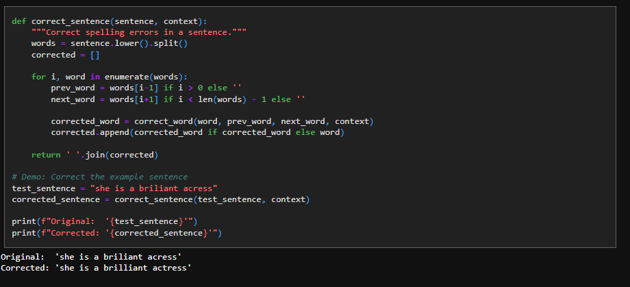
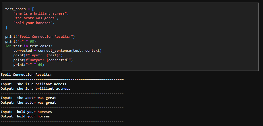
11. Sentence Correction
We use the correct_word mechanism to extend it to sentence level to get the spell correction to work:
12. Future Work
Peter Norvig runs his spell checker to some test datasets. I’ve consumed all the time I have allocated to this task as of now - but this will be interesting to performance tune at some point in the future.